Pivot tables are one of most powerful features of Microsoft Excel. A Pivot table is a data summarization tool that helps in extracting significance from a large amount of data. Pivot table can easily answer queries by allowing you to do basic data analysis.
We recently published a tutorial on VLOOKUP, another Excel feature that can help you in data analysis.
Like any other good spreadsheet software, Microsoft Excel also provides pivot table feature and it is very easy to use. All you need to do is to understand the concept of a pivot table. In this tutorial, we will explain how to use pivot table with the help of examples. You can download the sample Excel datasheet so that you can easily try the pivot table examples given below. This sample excel sheet contains data about the inventory of CDs in a movie shop.
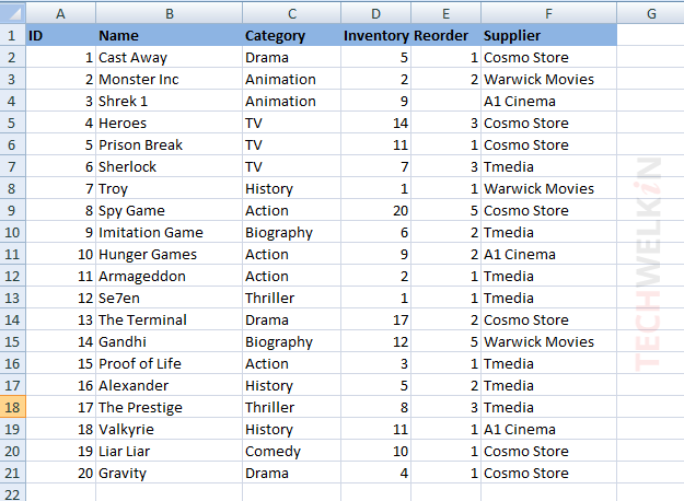
Sample Excel datasheet for movie store inventory
Insert a Pivot Table in Excel Sheet
To begin the tutorial, we will learn how to insert a pivot table in our sample Excel sheet.
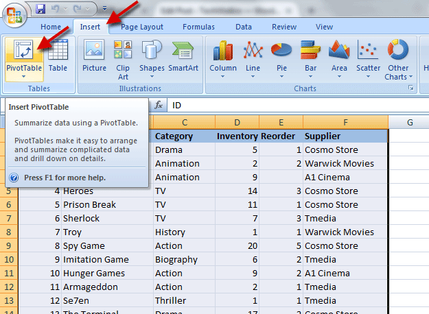
- Select all the data in the sheet. You should select header row as well.
- Go to Insert tab on Excel ribbon and click on PivotTable button.
- Create PivotTable dialog box will appear on screen. As you have already selected the data, Excel will automatically pick up the cell range. You will have the option for creating PivotTable in a new worksheet or in the existing worksheet. By default, PivotTable will be created in a new worksheet. We will take the default option.
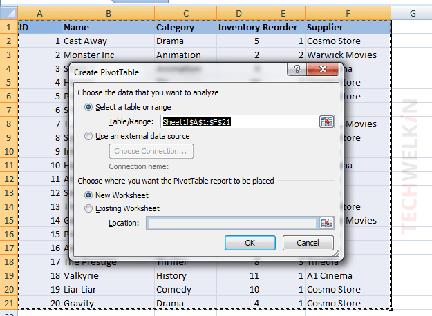
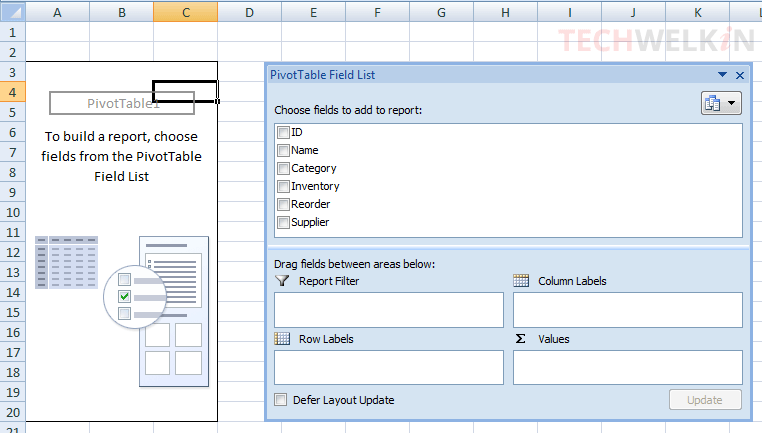
- Click OK button to insert a blank pivot table in a new worksheet. Besides blank pivot table, you will also see the PivotTable Field List dialog box. Please note that you may get this PivotTable Field List either as shown in the following image OR it could also appear docked on the right edge of the screen. Don’t worry, it’s one and the same thing!
NOTE: You may be wondering why Excel does not show a space between the words “Pivot” and “Table”. The reason is that Microsoft uses the compound word PivotTable as a trademark. The term Pivot Table (with a space) is a generic term and any software or vendor can use it but PivotTable™ is a trademark of Microsoft Corporation in the United States.
Adding Fields in Pivot Table
Now that we have created a blank pivot table, it is time to add required fields in this table. Before we do that, we need to understand what we want from our pivot table. So, let’s pose a question!
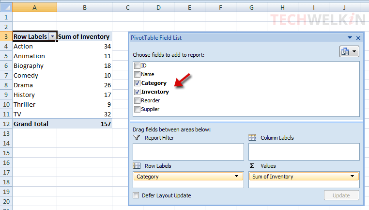
Let’s say, we want to know the total number of movie CDs we have under each category. For example, we want to know how many CDs we have under the Action category. Similarly we want to know the sum for all the movie categories. Can pivot table answer this question? Yes, of course! And you would be surprised how easy it is!
Just select Category and Inventory fields from the Choose fields to add to report box. And that’s it! You’ll see that both these fields have been added to the blank pivot table and the Inventory has been summed up according to category!
If you click on the dropdown arrow in the Row Labels cell, you can sort the rows and also hide/show any of them.
This was easy, wasn’t it? Now let’s see what else pivot table can do for us.
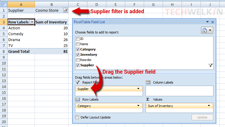
Another question for our pivot table. We want to see the Category-wise sum of inventory where Supplier‘s name is Cosmo Store. So, basically we want to know how many CDs purchased from Cosmo Store are still available under each category.
For this, we just need to add a filter in our pivot table
Adding Filter in Pivot Table
- Drag the Supplier field from the Choose fields to add to report box into the Report Filter box
- A filter will be added on top of the pivot table. You will see, now the pivot table has only four rows showing Categories. This means that Cosmo Store supplies CDs only in Action, Comedy, Drama and TV categories. Total number of CDs available in inventory is also being shown.
- In case, you want to know the same data from another Supplier, you can change the supplier name and the pivot table will automatically be refreshed. For this just click on the funnel icon in the cell showing Cosmo Store filter. You will get a list of all the Suppliers. Select the one you want to use.
Using Pivot Table with Functions like Count, Average, Min, Max etc.
It’s not that pivot table can only do summation for you. Pivot table can summerize data using the following Excel functions:
- Sum
- Count
- Min
- Max
- Average
- Product
- Count Numbers
- StdDev (standard deviation)
- StdDevp
- Var
- Varp
With the help of Min function, for example, we can easily find out the minimum inventory available for Supplier. This can help us in reordering the items.
- Clear everything from pivot table by unticking all the fields from Choose fields to add to report box. The pivot table will be blank again
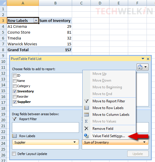
- Now tick Supplier and then Inventory fields in Choose fields to add to report box.
- Click on the Sum of Inventory in the Values box.
- Select Value Field Settings… option from the popup menu.
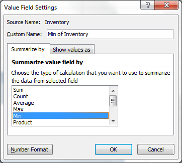
- Value Field Settings dialog box will appear. In this dialog box, you can select any of the summerization function you need. We will select Min function in order to answer our query.
- Click OK button and the pivot table will be updated with new information.
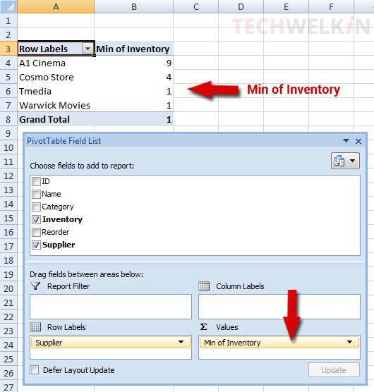
Here we can see in the pivot table that the minimum available items from Tmedia is 1 and from Cosmo Store 4 items are available. The question is answered!
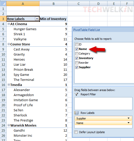
Show more information in Pivot Table
We can add more information in our pivot table to make it more meaningful. In the previous example, we found the minimum number of available inventory from each of the Supplier. But the above answer does not tell us which movies the minimum inventory belongs to. We see that Tmedia’s minimum inventory is 1. So, we should call Tmedia and reorder from them; but we don’t know which movie this “1” belongs to. So, we don’t know which movie is to be reordered.
To sort this out, we need to display more information in our pivot table. We need to add the Name field as well. So, we do that by simply ticking the Name field in the Choose fields to add to report box. And the new information would be instantaneously added to the pivot table.
What We Learnt From This Pivot Table Tutorial?
- Pivot table is a data summerization tool.
- Pivot table helps us in analyzing and draw required results from a big data set.
- Pivot table in Excel can summerize data using Sum, Count, Min, Max, Average, Product, Count Numbers, StdDev, StdDevp, Var and Varp functions.
- We can drag and drop fields in a pivot table.
- Pivot table essentially “pivots” or rotates the data around. That’s why the name.
- Compound word PivotTable is a trademark of Microsoft Corporation in USA.
To better understand the utility of pivot tables, let’s take another example. The following data sheet has been taken from Wikipedia:
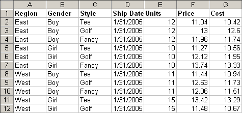
This data sheet is pretty flat and it does not offer any useful information. But when we pivot this table, we get a simpler table that summerize and simplify the data. For our eyes the following pivoted table is more meaningful as it tells us how many units were shipped on a particular date to various regions.
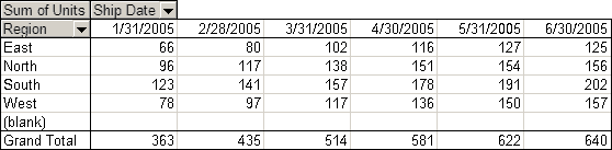
From this, we learn that an Excel sheet contains flat data… pivoting turns the flat data into information that we can use to make decisions.
We hope this tutorial on pivot tables in Excel was useful for you. If you have any questions on this topic, please feel free to ask through the comments section. We will try our best to assist you. Thank you for using TechWelkin!
Good. Thank you.