Sorting data is one of the most basic tasks when we work in spreadsheet software like Microsoft Excel. Sorting allows us to rather easily see pattern in a set of statistics. Sorting helps in data analysis and data organization. An Excel sheet stores data in rows and columns. Excel provides a number of methods to sort data columns. In this tutorial, we will learn how to sort data in Excel and we will also examine and solve the common problems in data sorting.
In Excel, you can sort text, numbers, date and time. But Excel goes beyond this and also allows you to sort data by cell color, font color and custom list etc. It is also possible to sort rows in Excel.
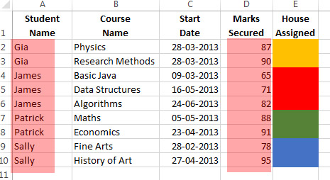
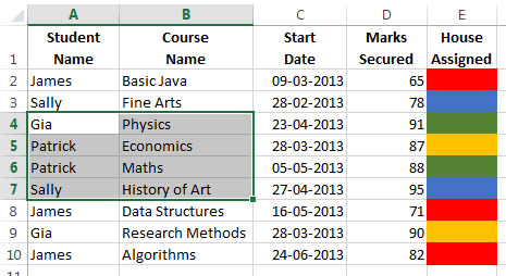
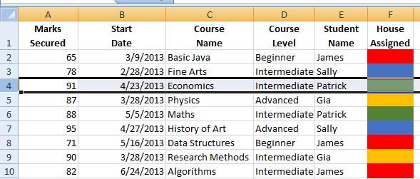
In the following tutorials, we will use a sample Excel datasheet. You can download this sheet so as to follow the sort examples given below. This sheet contains sample data related to students of a class.
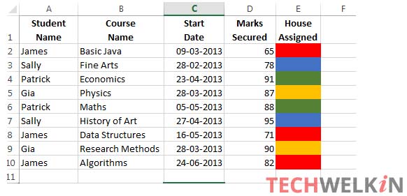
Sample Excel Data Sheet.
Quick Sorting Excel Data
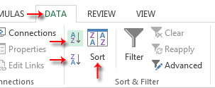
Before we plunge into any fancy sorting, let’s first understand how to quickly sort a column in Excel. There are buttons in Data tab (Sort & Filter group) for quickly sorting a column.
- Select the column that you want to sort
- Go to Data tab
- In Sort & Filter group, you will see two buttons: A to Z (for ascending sort order) and Z to A (for descending sort order). Ascending order will sort data from smaller to higher values. Descending order will sort data from higher to smaller values.
Sort options in Data tab of Excel.
- Click on either of these two buttons as required and the selected column will get sorted accordingly.
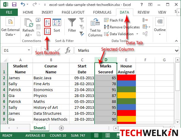
Sort in Excel. Quick sort buttons.
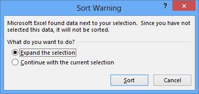
Sort Warning
When you do quick sort in Excel, chances are that you will receive a sort warning. This warning is very important and you must understand what it says otherwise your data may become inconsistent. The warning reads like:
Microsoft Excel found data next to your selection. Since you have not selected this data, it will not be sorted. What do you want to do? (1) Expand the selection. (2) Continue with the current selection.
Here Excel is trying to advice you that you should expand your selection. Since you’ve selected only one column, and if only that column gets sorted —then the overall data will become meaningless. Actually, you should select all the data (i.e. all the columns) while using sort command. But if you don’t select all the columns, Excel will warn you.
TIP: to quickly select all the data, select any cell within the data and then press Ctrl+A.
In most cases you’ll need to select the “Expand selection” option. Excel will automatically select all the columns adjacent to the column you had selected. Then Excel will sort the column selected by you and also change data in other columns to preserve the data integrity.
Sort warning in Excel.
Only in rare cases you would want to use the second option of “Continue with the current selection”. So, be careful here!
Sort the Whole Excel Sheet
- Select the column on which you want to be sorted
- Go to Data tab and click on the A to Z button to sort from smaller to bigger sort; or click on the Z to A button for bigger to smaller sort
Sort options in Data tab of Excel.
- Excel may show you sort warning. If it does, select “Expand selection” option and click OK
- The whole sheet will be sorted.
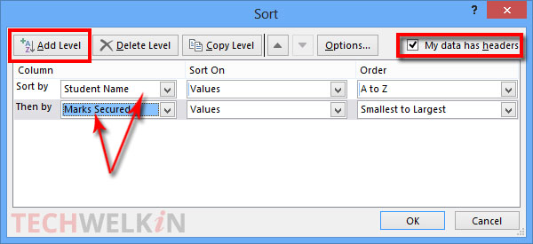
Sort Two or More Columns
More often than not, we need to sort two or more columns in Excel. For example, we may want to sort Student Name column and then sort Marks Secured column. What we want here is that first all the student names should get alphabetically sorted and then the Marks Secured column should get sorted.
- Select the columns that you want to sort
- Go to Data tab and from Sort & Filter group, click on the Sort button
Sort options in Data tab of Excel.
- Sort dialog box will appear
- Select the first column name to be sorted from the Sort by dropdown list
- Select Values from Sort on dropdown list
- Select required order from Sort order dropdown list
- Now click on Add Level button to add more columns. Select the appropriate column name, sort on and order options
- Click OK to complete the process
Excel sort options.
In our example, the datasheet has been sorted by Student Name and then by Marks Secured columns.
Excel sheet sorted on two columns.
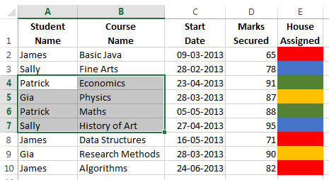
Sort a Cell Range
Excel allows you to sort not only the entire column but also a selected cell range. Sometimes you may want to sort only a portion of columns. For this you can select a cell range and do the required sort within that cell range.
- Select a cell range (in our example, we are selecting A4:B7)
Selected cell range for sorting.
- Click on the Sort button in the Data tab.
Sort options in Data tab of Excel.
- The Sort options dialog box will come up. First of all, unselect the My data has headers checkbox. If this is selected, Excel will not consider the first row in selection for sorting. It will assume that the first row in selection contains header names therefore will omit them from sorting. But we want our whole selected cell range to be sorted. So, we unselect My data has headers checkbox. We want to sort both the columns in our selected cell range (A4:B7), so we set the sort options for both the columns.
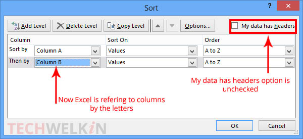
Sort dialog box with “My data has headers” option unchecked.
- Click OK and the cell range will be sorted. See the results in the image given below.
Sorted cell range.
As you can see, names of students are sorted and then course names are are also sorted.
CAVEAT: You should be careful while sorting a cell range. As you can see, the above sort process has made the overall data in rows wrong! Gia who had actually scored 87 marks in Physics, now has 91 marks in that subject. This happens because Excel has sorted only the selected cell range. The adjacent data remained unmoved while the data in cell range changed due to sort function. So, be careful and sort a cell range only when you know what you’re doing. Mostly such sorting is done only to be undone. Usually people sort a cell range to see the result and then press Ctrl+Z to undo such sorting.
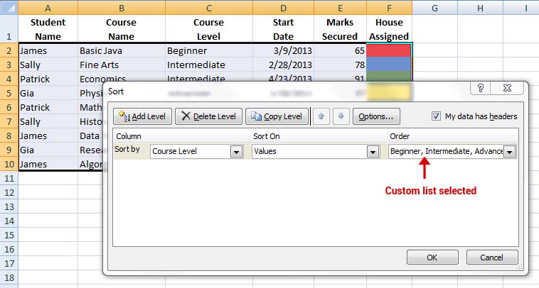
Create Your Own Sort Order With Custom List…
This is very interesting facility provided by Excel. We have seen that Excel can sort data in ascending or descending order. But sometimes we do not want to sort our data with the regular definition of order. We want to create our own custom order and then sort the data with this custom order. To demonstrate this, we have added a new column in our sample data sheet. Name of this new column is Course Level. There are three possible values for the Course Level column; Beginner, Intermediate and Advanced. We have assigned the appropriate values to various student records. The updated data sheet now looks like this:
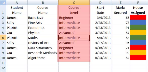
Updated datasheet
As we know, Beginner level comes first and then comes the Intermediate level. At the end Advanced level comes. But if we alphabetically sort this data on Course Level column, the sort order would be Advanced, Beginner, Intermediate. This is clearly not what we want! We want to sort data so that all the Beginner level rows come first followed by Intermediate rows and the rows with Advanced level should come in the end.
This is where custom sort can help us! Following example demonstrate how you can do custom sorting:
- First of all select any cell in the data and press Ctrl+A to select all the data.
- Go to Data tab and click on the Sort button to open Sort dialog box
Sort options in Data tab of Excel.
- As we have explained before, select the column name from the Sort by dropdown list. Then from the Order dropdown list select Custom List… option.
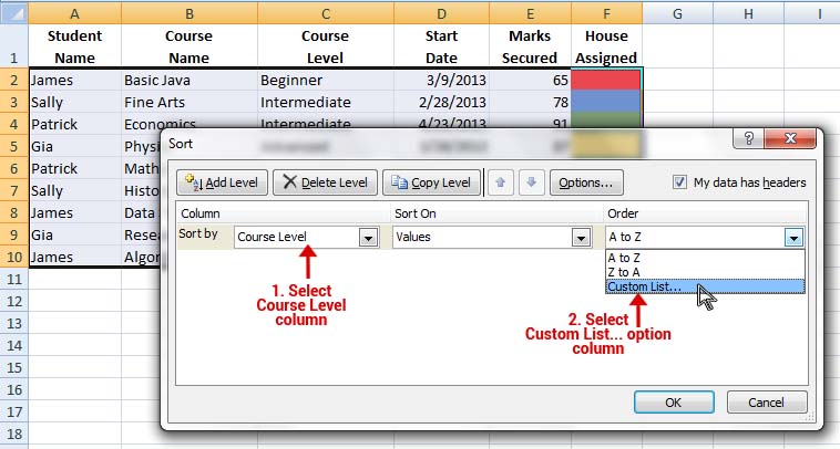
Custom list option in the Sort dialog box.
- When you will select Custom List… option, a new box will open. In this Custom List dialog box, you should type your custom order in the box given on the right hand side. Type first item, then press ENTER key, then type second item and so on. Make sure that while you’re typing, NEW LIST is selected in the left hand side box. Remember, your list should be in exactly the same order that you want Excel to follow while sorting.
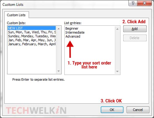
Making custom list in Excel.
- After typing the list, click on Add button to add the newly typed list in the custom lists. You’ll see that the new list items will add to the left box. Now click on OK button. Voila! Your new custom order has been added to the Order dropdown list.
Custom list has been selected for sorting.
- Now click OK button to complete the sort process. And the results will be just as we wanted! The Course Level column has been sorted according to the newly defined custom order. Rows with Beginner come first. Then come the rows with Intermediate and rows with Advanced course level come in the end.
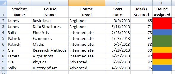
Course Level column has been custom sorted.
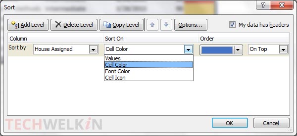
Sort by Cell Formatting in Excel
Yet another great facility provided by MS Excel is that you can sort a column on the basis of the cell formatting. For example, you can ask Excel to sort by cell color or font color or cell icon. To give you a demonstration of this feature, we will sort our sample datasheet by House Assigned column. This column contains cells of various colors which represent the House to which a student is associated.
Let’s say we want to see on top all the rows where student belongs to the Blue house.
- Select any cell in the data and press Ctrl+A to select all the data.
- Go to Data tab and click on the Sort button.
Sort options in Data tab of Excel.
- The Sort dialog box will open. From the Sort by dropdown list, select House Assigned column. From the Sort on dropdown list, select Cell Color.
Sort by cell color option in Sort dialog box.
- As soon as you will select Cell Color, you will see that the Order option will begin to show a lost of all the cell colors that are present in selected column.
- Select blue from the color list and then select whether you want to see the blue rows on top or on bottom. In our example, we have selected On Top. Click OK and the data will be sorted with blue rows appearing on top.
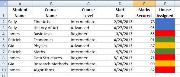
Data sorted by cell color.
Similarly, you can also sort data by Font Color and Cell Icon.
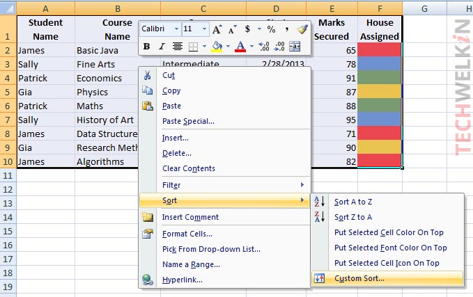
How to Sort by Rows in Excel
So far we have seen various methods of sorting Excel data by columns. But is it possible to sort Excel data by rows? Yes! You can easily sort data on the basis of rows and the steps are almost same as in case of sorting columns. Sorting by rows means that the process is done from left to right instead of top to bottom. We can also choose between ascending and descending order. If we select ascending order, then the smallest value will be found of the left-most side and the biggest value will be on the right-most side. Descending order will be opposite of this.
- Select any cell in the data and press Ctrl+A to select all the data.
- Take right click anywhere in the selected range and choose Sort > Custom Sort from the popup menu. The Sort dialog box will appear. Note that this right-click method is an alternative way for bringing up the same Sort dialog box.
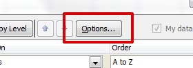
- Click on the Options… button in the Sort dialog box
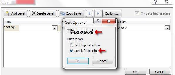
- Another tiny box will appear on your screen. Here you can select if you want to sort data from top to bottom or left to right. Because we want to sort but rows, select Sort left to right option. You can also select whether you want sort operation to be case sensitive or not. After making choices, click OK.
- Now select which row you want to Sort by and then click OK. Well, of course, you can also make choices of Sort on and Order if you need to.
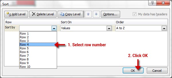
- Here is the result! Data has been sorted by Row 4. Rest of the data has been moved around by Excel to keep the integrity of data intact.
More Tips for Excel Data Sort
- If you have hidden any rows or columns, you should unhide them before sorting. The hidden rows/columns are not moved when sorting is done. Therefore, if you will unhide rows/columns after sorting then the data will become inconsistent.
- Sort order depends on the locale setting in your computer. Different languages have different locales and their alphabets may have different sorting order. So, if you work on an English language computer, and you’re sorting Hindi or Chinese data in Excel, you should know that the sort order of these languages may be different.
- It is always better to have the first row as header row and while sorting data, you should keep the My data has headers option turned on. By default Excel keeps this option turned on. A header row makes the data easier to read and understand. If My data has headers option is turned on, then Excel will not include the first row in sorting operation.
- If you have a header row: Data tab > Sort & Filter group > Sort button > Tick the My data has header checkbox in Sort dialog box.
- If you don’t have a header row: Data tab > Sort & Filter group > Sort button > Untick the My data has header checkbox in Sort dialog box.
- Although Ctrl+A is a really nice and quick way of all the selecting data, but still you should take a closer look and confirm that all the intended data has been selected before you proceed with the sort function.
- If the data you are about to sort contains a cell with a formula, it is possible that sorting will change the formula results because of change in cell references. You should recalculate the formula after sorting.
We hope that this article on sorting of Excel data was helpful for you. Although sorting is a simple and often used function, still there could always be new things that you can learn about simple procedures! Should you have any questions regarding this topic, please feel free to ask in the comments section. We will try our best to assist you. Thank you for using TechWelkin!
Quote “Only in rare cases you would want to use the second option of “Continue with the current selection”. So, be careful here!”
Assumption based on the same often incorrect premise as Excel itself. You have made the assumption that Excel is being used for one purpose – to hold cells that have linked data – which is NOT necessarily correct. This function should be able to be set in options, as it is a total time waster to those who have to continually reset the incorrect default, every search.
Excel spreadsheet has a total of 88 rows of data, 8 columns wide. I select a priority of sorting using 3 columns. The system will sort the top 61 rows correctly, but then also does a similar sort of the bottom 27 rows, which are done correctly but are not merged in with the top 61 rows.
What can I do to correct this situation?
Tks
Allen