At first glance, for most people, the SUMPRODUCT formula of Excel may look “nice but useless”. However, there are situations when SUMPRODUCT turns out to be a very useful Excel formula. The meaning of SUMPRODUCT is the sum of products —the function does exactly what it says! This formula first multiplies various pairs of values and then sum up all the results. Here is an example:
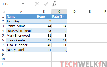
In the above image, we may want to calculate the total payment to be made to all the employees. To do this, first we will have to multiply hours and rate and then add all the multiplication results. SUMPRODUCT is a function that can do all this very easily. In this tutorial, we will explain how to use SUMPRODUCT function.
Syntax of SUMPRODUCT in Excel
=SUMPRODUCT(array1, [array2], [array3], …)
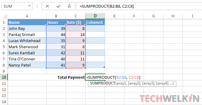
SUMPRODUCT function takes one or more arrays as arguments. In Excel these arrays are basically cell ranges. Providing first array is mandatory and other arrays are optional. Let’s use this function to calculate the total payment to be made as shown in the above example.
- Select a cell where you want to show the result (we will use D10 for result)
- Type formula =SUMPRODUCT(B2:B8, C2:C8)
- Press Enter key and you will get 2762 as result
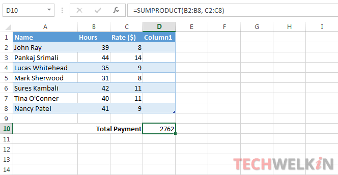
This result is achieved as (39*8 + 44*14 + 35*9 + …. 41*9 = 2762)
Another Example
We can also use conditional SUMPRODUCT. This formula will first do a search like VLOOKUP and then will add up the results. Let’s assume that we want total payment only for those employees whose pay rate is over $10 and hour. For this we can use the following formula:
=SUMPRODUCT((C2:C8>10)*B2:B8,C2:C8)
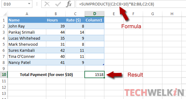
The result will be 1518. Here the function will first lookup the values in column C where rate is over $10 and then it will multiply those values with corresponding values in column B.
Problems and Errors in SUMPRODUCT
#VALUE Error: The function shows #VALUE error when the arrays supplied as arguments are not of the same dimensions. This means that the number of items and dimensions must be same in all the cell ranges that you pass as arguments. Following formula will throw #VALUE error:
=SUMPRODUCT(B2:D8, C2:C8)
The error comes because first cell range B2:D8 is bigger than the second cell range C2:C8
Unexpected results: If any of the cell in the provided arguments contains a non-numerical value, then SUMPRODUCT will assume that that cell contains zero. When zero is multiplied with any number the result would be zero and thus the overall result of SUMPRODUCT will be wrong. So, you must make sure that all the cells contain only numeric values.
We hope that this tutorial was helpful for you in understand the SUMPRODUCT formula and its usage. If you have any question regarding this formula, please feel free to ask through comments section. We will try our best to assist you. Thank you for using TechWelkin!
Leave a Reply